Quantization of Models: Why and How

When storing data in memory, the data type used to represent the data has an impact on the memory usage and the performance of the overall system. Consider saving a number. On a high level, the number can either be an integer (whole number) or a floating-point number (number with decimal). Floating-point numbers can represent larger range of numbers with higher precision. Weights and biases in a large language model, which are learned during training and are used to make predictions, are stored as floating-point numbers to maintain high precision. The count of these parameters is what constitutes the size of the model, memory usage and how much computational resources are needed to run the model. In this post, we'll discuss how quantization can be used to reduce the memory usage of models and improve performance (assuming the loss of precision is acceptable). Quantized models can be used to run on devices or environments with limited computational resources, such as mobile or in the browser.

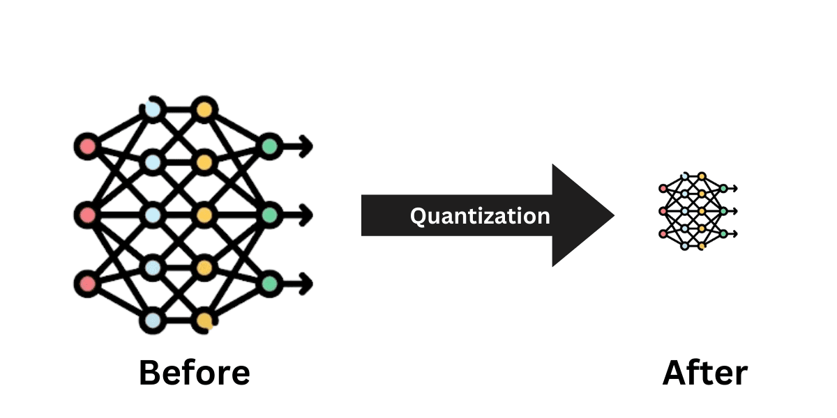Abstract representation of Quantization

These weights and biases are the core of the model and are stored as 2 or 3-dimensional arrays. For example, here's a 3-dimensional representation of a 3x3 matrix:

[
  [  0.9876,   0.1111,   0.2567 ],
  [  1.2345,  10.1234,  -0.9999 ],
  [  5.4321,   0.0012,  -2.3456 ]
]

Assuming each of these numbers is stored as a 32-bit floating-point number, the total memory usage for this matrix is 36 bytes (3x3x4).

Quick note about the floating point number representation:

Floating-point numbers are represented using the IEEE 754 standard. The standard defines the format of the number, which includes the sign bit, exponent, and mantissa. The sign bit represents the sign of the number (positive or negative), the exponent represents the scale/range of the number, and the mantissa represents the precision of the number. For example, a 32-bit floating-point number has 23 bits for the mantissa, while a 16-bit floating-point number has 10 bits for the mantissa.

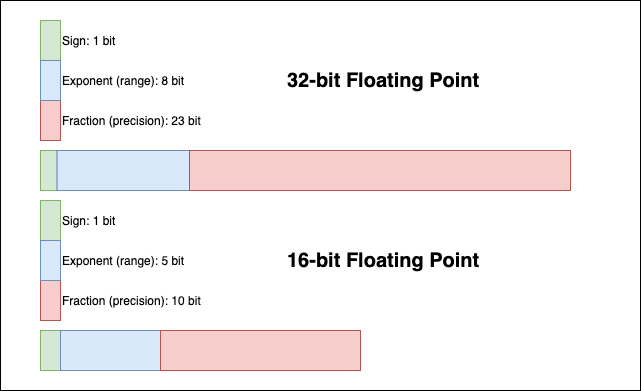Floating point representation

Going back to the matrix, if this data is converted to 16-bit floating-point numbers, the total memory usage would be 18 bytes (3x3x2). This is half the memory usage compared to 32-bit floating-point numbers. Here's the what the matrix would look like in 16-bit floating-point numbers:

[
  [  0.9873,   0.1111,   0.2566 ],
  [  1.2344,  10.1250,  -0.9995 ],
  [  5.4321,   0.0012,  -2.3457 ]
]

If we stored this in 8-bit integers, the total memory usage would be 9 bytes (3x3x1).

[
  [  1,  0,  0 ],
  [  1, 10,  0 ],
  [  5,  0, -2 ]
]

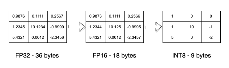Size difference after down casting

Yes, there's a loss of precision. But whether it matters or not is dependent on the use case the data is being used for. For example, for a model used to do financial forecasting, high precision is crucial as a small change in numbers can lead to a large difference in the forecasted value. However, a model used for vacation planning can afford to lose some precision to save memory and improve performance. Using low precision data can significantly reduce the memory usage and improve the performance of the model. It also allows the model to be deployed on devices with limited computational resources. Memory is cheap but computational resources can be expensive. GPUs and TPUs consume a lot of power. The reason GPUs are needed for training and inference is because they can perform a large number of operations in parallel on large amounts of data. By reducing the memory usage, the model can be run for inference on devices with limited computational resources, such as mobile phones and IoT devices.

On a high level, quantization is the process of converting high precision data to low precision data.

The following code demonstrates how to quantize using PyTorch and compare the memory usage of the original and quantized tensors. I ran this code on a ubuntu22 image with Python 3.10. Ensure you install the pip packages before running the code.

numpy<2.0
transformers==4.35.2
torch==2.1.0
accelerate==0.24.1
datasets
evaluate
scikit-learn

import time

import torch
from transformers import AutoModelForSequenceClassification, AutoTokenizer
from datasets import load_dataset
from evaluate import load

# Load model.
# distilbert-base-uncased-finetuned-sst-2-english is a small model for sentiment analysis.

model_name = "distilbert-base-uncased-finetuned-sst-2-english"
model = AutoModelForSequenceClassification.from_pretrained(model_name, num_labels=2)
tokenizer = AutoTokenizer.from_pretrained(model_name)
sample_count = 500

# Check Original Model Size
# Each parameter in FP32 uses 4 bytes.
original_size_mb = sum(p.numel() for p in model.parameters()) * 4 / (1024 * 1024)
print(f"Original Model Size: {original_size_mb:.2f} MB")

# https://gluebenchmark.com/
# GLUE benchmark is a collection of multiple (NLU) tasks to evaluate and compare the performance of different language models
# Within GLUE, SST-2 (the Stanford Sentiment Treebank version 2) is a sentiment analysis task where each sentence from movie reviews is labeled as either positive or negative.
dataset = load_dataset("glue", "sst2", split="validation[:" + str(sample_count) + "]")
metric = load("accuracy")

def evaluate_model(model, tokenizer, dataset, metric):
    model.eval()
    all_preds, all_labels = [], []
    for item in dataset:
        inputs = tokenizer(item["sentence"], return_tensors="pt")
        with torch.no_grad():
            outputs = model(**inputs)
        # get the raw scores, pick the class (positive/negative) with the highest score, and convert the result to a list.
        preds = outputs.logits.argmax(dim=-1).cpu().numpy().tolist()
        all_preds.extend(preds)
        all_labels.append(item["label"])
    return metric.compute(predictions=all_preds, references=all_labels)

# baseline stats
start_time = time.time()
baseline_metrics = evaluate_model(model, tokenizer, dataset, metric)
baseline_time = time.time() - start_time

print(f"Baseline Accuracy: {baseline_metrics['accuracy']:.4f}")
print(f"Baseline Inference Time: {baseline_time:.2f} seconds for {sample_count} samples")

# Post-Training Quantization (PTQ)
quantized_model = torch.quantization.quantize_dynamic(
    model, {torch.nn.Linear}, dtype=torch.qint8
)

# quantized model size
quantized_size_mb = sum(p.numel() for p in quantized_model.parameters()) * 4 / (1024 * 1024)
print(f"Quantized Model Size: {quantized_size_mb:.2f} MB")

# quantized stats
start_time = time.time()
quantized_metrics = evaluate_model(quantized_model, tokenizer, dataset, metric)
quantized_time = time.time() - start_time

print(f"Quantized Accuracy: {quantized_metrics['accuracy']:.4f}")
print(f"Quantized Inference Time: {quantized_time:.2f} seconds for {sample_count} samples")

# summary of stats
size_reduction = (1 - (quantized_size_mb / original_size_mb)) * 100
speedup = baseline_time / quantized_time if quantized_time != 0 else 1.0

print(f"\nSize Reduction: {size_reduction:.2f}%")
print(f"Speedup: {speedup:.2f}x")

# sample inference
sample_text = "I wouldn't necessarily call the food at the restaurant bad, but I wouldn't recommend it either."
inputs = tokenizer(sample_text, return_tensors="pt")

# with original model
with torch.no_grad():
    original_outputs = model(**inputs)
original_pred_label = original_outputs.logits.argmax(dim=-1).cpu().item()

# with quantized model
with torch.no_grad():
    quant_outputs = quantized_model(**inputs)
quant_pred_label = quant_outputs.logits.argmax(dim=-1).cpu().item()

label_map = {0: "Negative", 1: "Positive"}
print(f"\nSample Text: {sample_text}")
print(f"Original Model: {label_map[original_pred_label]}")
print(f"Quantized Model: {label_map[quant_pred_label]}")

Output from this code on my machine:

root@1bddc3738cb2:/apps# python qn.py

Original Model Size: 255.41 MB
Baseline Accuracy: 0.9120
Baseline Inference Time: 19.93 seconds for 500 samples
Quantized Model Size: 91.00 MB
Quantized Accuracy: 0.9020
Quantized Inference Time: 12.84 seconds for 500 samples

Size Reduction: 64.37%
Speedup: 1.55x

Sample Text: I wouldn't necessarily call the food at the restaurant bad, but I wouldn't recommend it either?
Original Model Prediction: Negative
Quantized Model Prediction: Negative

Notice the 1.5 time speedup and 64% reduction in model size. The accuracy of the quantized model is slightly lower than the original model. The loss in accuracy is acceptable for this use case. The quantized model is using 8-bit integers to represent the weights and biases. The quantized model is smaller in size and faster to run.

This is just a demonstration on a model that does sentiment analysis. We could save the quantized model and package it as a WASM (WebAssembly) module to run in the browser. The quantized model can be used to make predictions on the client side without needing to send the data to the server. This can be useful for privacy-sensitive applications where the data should not leave the client device.

Quantization can be done either during training or after training. What we did above is an example of post-training quantization. The code used above uses PyTorch's dynamic quantization.

Checkout SmoothQuant, a post-training quantization method for LLMS with a large number of parameters that uses a smooth quantization technique to reduce the loss in accuracy.

Let me know if you've used quantized models in your projects, what use cases you've used them for, and what challenges you faced.